scATrans without spliced/unspliced layers: differential expression + enrichment + plotting

This tutorial is for the majority of scRNA-seq users who do not have RNA velocity (spliced/unspliced) layers — just an ordinary count matrix from 10x, Smart-seq, or any other protocol. Everything below uses scat.differential_expression(...) instead of scat.active_score(...), and never touches a spliced/unspliced/mature/nascent layer. The exact same code works unmodified on a plain count-matrix .h5ad with no velocity layers at all.

For the velocity-aware active_score workflow on the same dataset, see the sibling tutorial Active Transcription Scoring on Real Spinal Cord Injury Data.

Dataset

We use EC.h5ad: endothelial cells (EC) subset from a real mouse spinal cord single-nucleus RNA-seq dataset, comparing uninjured controls (UN, 3 replicates) against spinal cord injury (SCI, 3 replicates):

Squair, J.W., Gautier, M., Kathe, C., et al. (2021). Confronting false discoveries in single-cell differential expression. Nature Communications 12, 5692. DOI: 10.1038/s41467-021-25960-2. GEO: GSE165003.

See References & Data Sources for the full citation list. This paper is itself about pseudoreplication and false-discovery risk in single-cell DE — fitting context for this tutorial, which reports real, sometimes non-significant results below rather than a cherry-picked toy example (small-n designs like this 3-vs-3 comparison commonly have limited genome-wide DE power; see Statistical Guidance & Reporting Checklist).

differential_expression and active_score share the same downstream tooling — filter_active_genes, all scat.pl.* plots, and every enrichment function — the only difference is that differential_expression skips the unspliced-excess term entirely.

%matplotlib inline

import sys
sys.path.insert(0, "../../src")  # use the in-repo scatrans, not any installed copy

import warnings
warnings.filterwarnings("ignore")

import scanpy as sc
import scatrans as scat

print("scatrans:", scat.__file__)

scatrans: /home/lieber/scATrans-main/docs/tutorials/../../src/scatrans/__init__.py

Load and inspect

We deliberately only ever look at adata.X (raw counts) below — no layers access anywhere in this notebook.

adata = sc.read_h5ad("../../EC.h5ad")
adata

AnnData object with n_obs × n_vars = 177 × 26451
    obs: 'n_genes_by_counts', 'log1p_n_genes_by_counts', 'total_counts', 'log1p_total_counts', 'pct_counts_in_top_50_genes', 'pct_counts_in_top_100_genes', 'pct_counts_in_top_200_genes', 'pct_counts_in_top_500_genes', 'condition', 'sample', 'GSM_ID', 'total_counts_mt', 'pct_counts_mt', 'n_genes', 'doublet_score', 'predicted_doublet'
    var: 'gene_symbol', 'mt', 'n_cells_by_counts', 'mean_counts', 'pct_dropout_by_counts', 'total_counts', 'n_cells'
    uns: 'sample_colors', 'scrublet'
    layers: 'ambiguous', 'mature', 'nascent', 'spliced', 'unspliced'

adata.obs[["condition", "sample", "GSM_ID"]].value_counts().sort_index()

condition  sample  GSM_ID    
SCI        rep1    GSM5024314    35
           rep2    GSM5024315    23
           rep3    GSM5024316    37
UN         rep1    GSM5024317    27
           rep2    GSM5024318    38
           rep3    GSM5024319    17
Name: count, dtype: int64

QC and light filtering

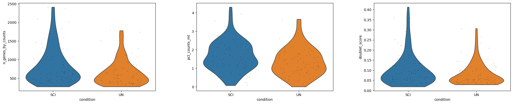
This EC subset was already QC’d upstream (doublet scores, mito %, and gene counts are precomputed in .obs). We apply the same filters here for completeness / robustness — on this dataset they happen to remove zero cells, since the upstream authors already excluded low-quality cells.

n0 = adata.n_obs
adata = adata[~adata.obs["predicted_doublet"]].copy()
adata = adata[adata.obs["pct_counts_mt"] < 20].copy()
adata = adata[adata.obs["n_genes_by_counts"] > 200].copy()
sc.pp.filter_genes(adata, min_cells=3)
print(f"cells kept: {adata.n_obs} of {n0}")
print(f"genes kept: {adata.n_vars}")

cells kept: 177 of 177
genes kept: 9221

sc.pl.violin(
    adata, ["n_genes_by_counts", "pct_counts_mt", "doublet_score"],
    groupby="condition", jitter=0.3, multi_panel=True,
)

Preserve raw counts, then preprocess

store_raw_counts snapshots .X into layers["counts"] (and .raw) before any HVG/normalize/log1p step — this is what lets enrichment functions later auto-supply the correct measured-gene background via adata=. Count-based DE backends (PyDESeq2, Memento) need these raw integer counts; the de_preprocess="auto" step inside differential_expression also uses the .uns["log1p"] marker scanpy sets to detect whether .X is already log-normalized (see Standalone Differential Expression (no velocity data required) for the anndata.concat() caveat around this marker).

scat.store_raw_counts(adata, layer="counts", save_raw=True)

adata_norm = adata.copy()
sc.pp.normalize_total(adata_norm, target_sum=1e4)
sc.pp.log1p(adata_norm)

Backend A: single-cell Wilcoxon DE

The simplest, fastest path: scanpy’s rank_genes_groups directly on log-normalized single cells.

adata_norm, de_wilcoxon = scat.differential_expression(
    adata_norm,
    groupby="condition",
    target_group="SCI",
    reference_group="UN",
    de_method="wilcoxon",
    de_preprocess="none",  # we already normalized + log1p'd above
)
de_wilcoxon.sort_values("logFC", ascending=False).head(10)

WARNING: It seems you use rank_genes_groups on the raw count data. Please logarithmize your data before calling rank_genes_groups.

	logFC	p_val	p_adj	baseMean
Tpcn1	27.242462	0.227766	0.9938	0.116235
Prdm16	27.127773	0.334591	0.9938	0.118895
Pgls	27.004536	0.227766	0.9938	0.126359
Nxn	27.004536	0.227766	0.9938	0.137124
Gm57952	27.004536	0.227766	0.9938	0.124299
Rab11fip1	27.004536	0.277691	0.9938	0.103826
Dmtf1	27.004536	0.147796	0.9938	0.125101
Pacsin2	26.871260	0.334591	0.9938	0.104579
Kcnj10	26.871260	0.227766	0.9938	0.122506
Plcl1	26.871260	0.277691	0.9938	0.112288

print("min p_adj:", de_wilcoxon["p_adj"].min())
print("genes with p_adj < 0.05:", (de_wilcoxon["p_adj"] < 0.05).sum())

min p_adj: 0.9938003852887332
genes with p_adj < 0.05: 0

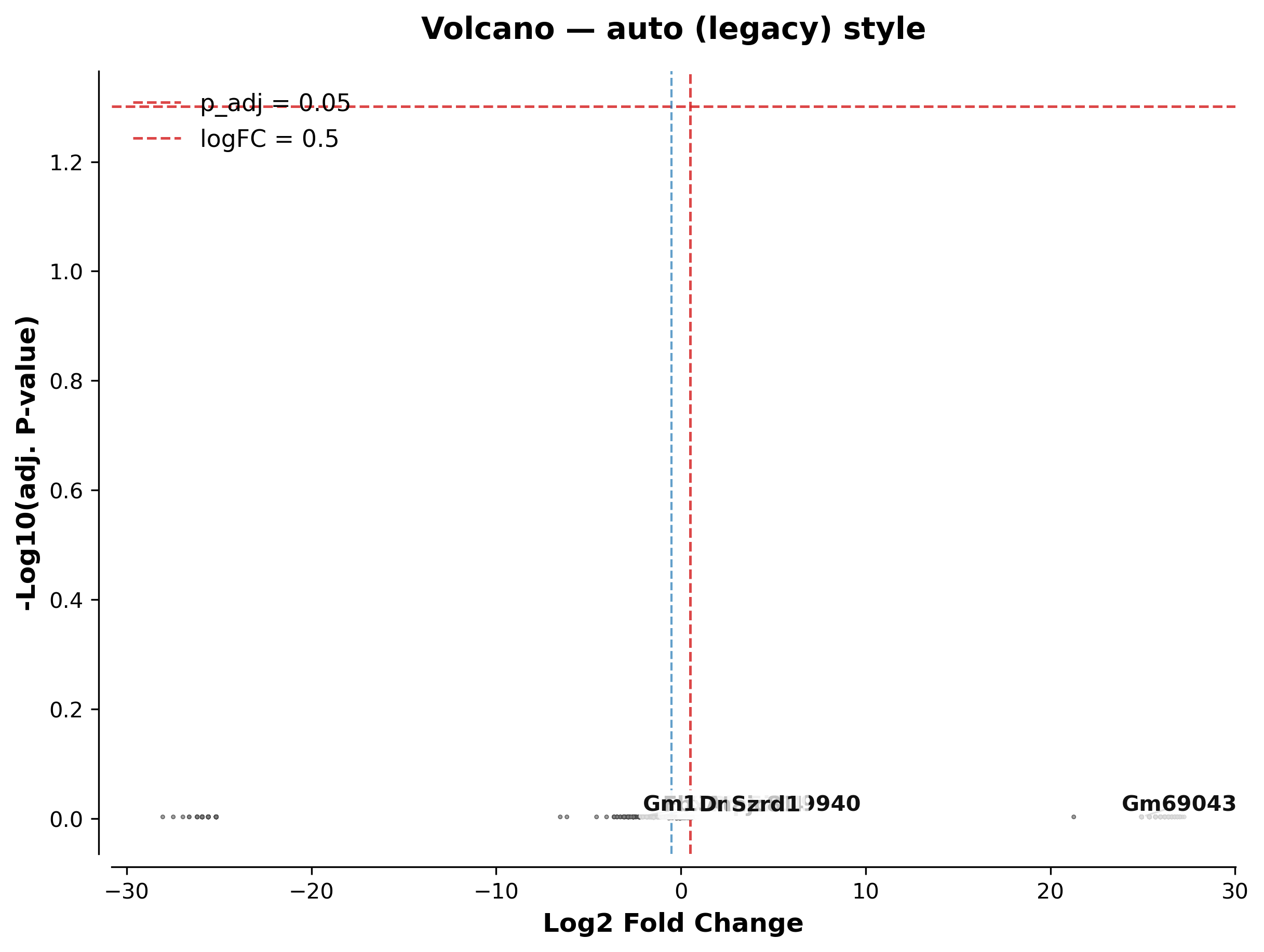
Note

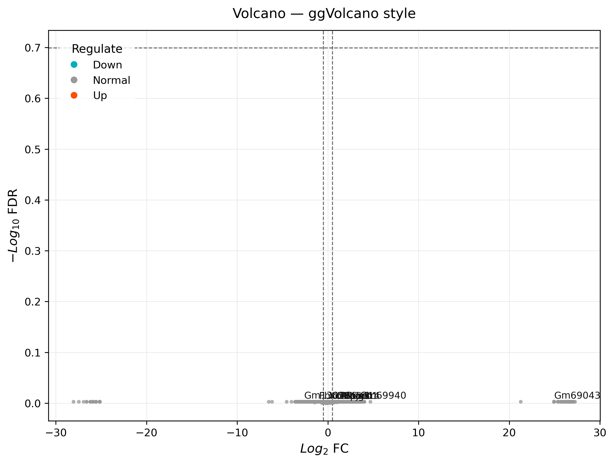
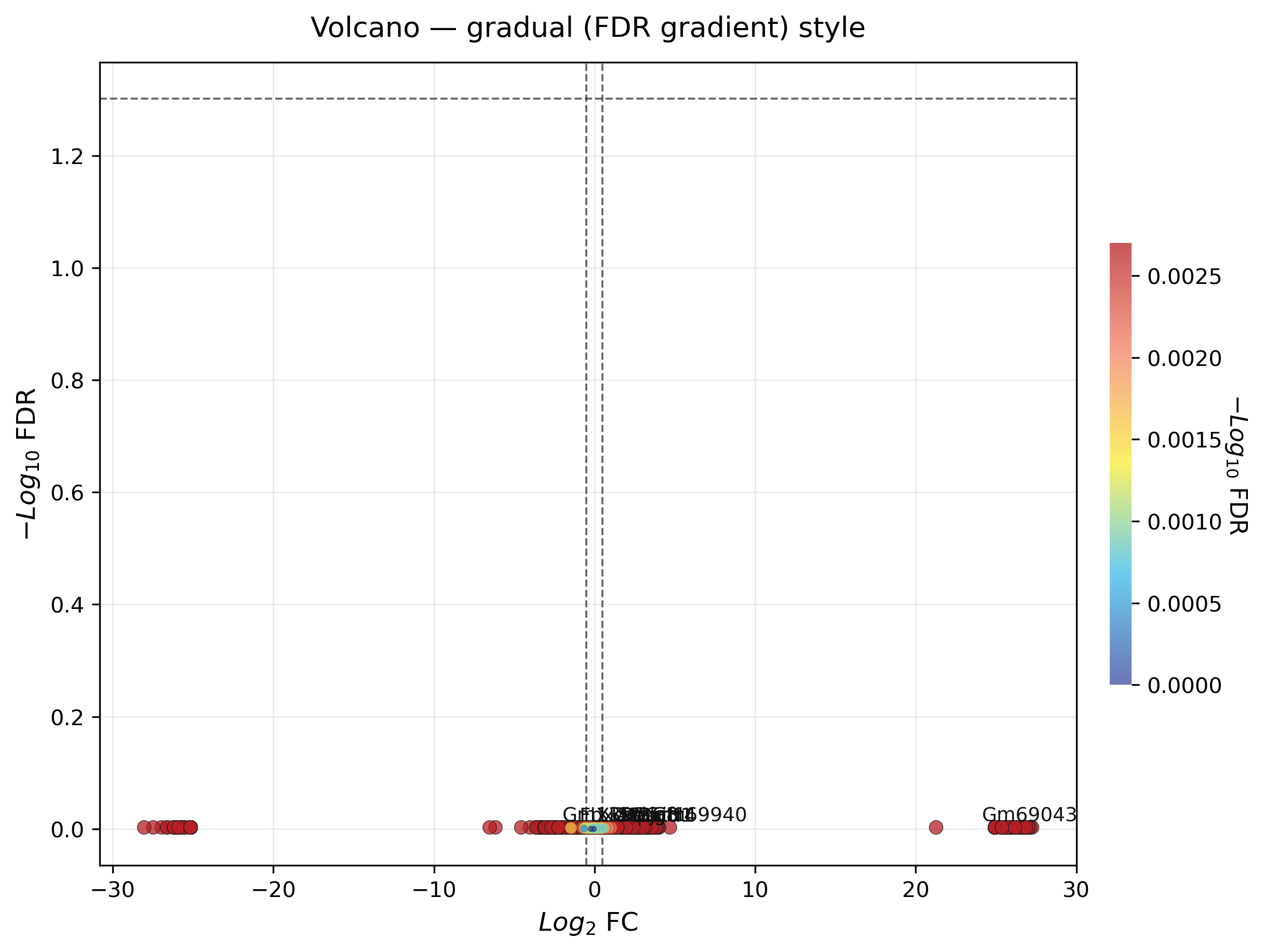
With only 3 replicates per condition, no gene reaches genome-wide p_adj < 0.05 here — this is real, honest small-n biology, not a bug. filter_active_genes with strict cutoffs legitimately returns very few or zero candidates. The practical workaround (used throughout this notebook) is to rank by nominal (unadjusted) p-value and effect size for hypothesis-generating candidate lists, and to say so explicitly rather than reporting p_adj < 0.05 claims that the data does not support. See Statistical Guidance & Reporting Checklist for the full reporting checklist.

candidates_strict = scat.filter_active_genes(de_wilcoxon, pval_cutoff=0.2, logfc_cutoff=0.3)
print("strict candidates (p_adj<0.2, |logFC|>0.3):", len(candidates_strict))

# Exploratory ranking: top 100 upregulated genes by nominal p-value
candidates = de_wilcoxon[de_wilcoxon["logFC"] > 0].sort_values("p_val").head(100)
print("exploratory candidates (top 100 upregulated by nominal p-value):", len(candidates))
candidates.head(10)

strict candidates (p_adj<0.2, |logFC|>0.3): 0
exploratory candidates (top 100 upregulated by nominal p-value): 100

	logFC	p_val	p_adj	baseMean
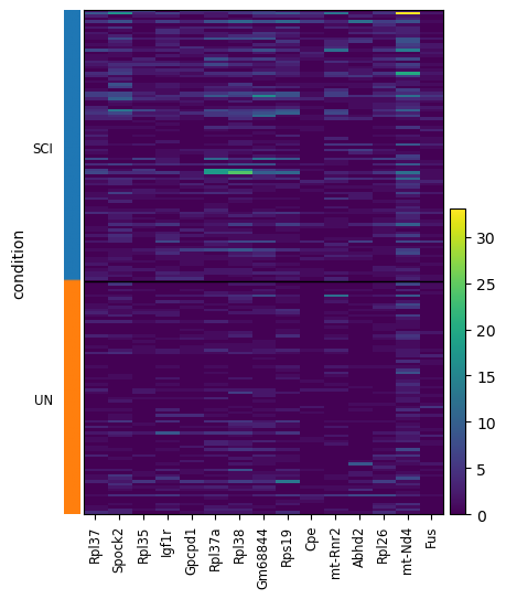
Rpl37	2.161662	0.000302	0.9938	1.468993
Spock2	2.577669	0.000312	0.9938	1.783297
Rpl35	2.087135	0.000397	0.9938	1.085354
Igf1r	1.444869	0.000446	0.9938	1.513025
Gpcpd1	1.772408	0.000603	0.9938	1.247660
Rpl37a	2.572021	0.001323	0.9938	1.647515
Rpl38	2.344653	0.001573	0.9938	1.909690
Gm68844	2.785950	0.001696	0.9938	1.732615
Rps19	1.891919	0.002009	0.9938	1.650908
Cpe	2.122542	0.002111	0.9938	0.719209

Backend B: pseudobulk + PyDESeq2

With 3 biological replicates per group, aggregating to pseudobulk and running count-based DESeq2 is the more defensible choice for a real publication (see the DE-backend decision guide in Core Workflow). We compare its top genes against the Wilcoxon single-cell result above — backend choice visibly changes which genes come out on top.

adata_pb = adata.copy()
adata_pb, de_pseudobulk = scat.differential_expression(
    adata_pb,
    groupby="condition",
    target_group="SCI",
    reference_group="UN",
    use_pseudobulk=True,
    sample_col="sample",
    pseudobulk_de_backend="pydeseq2",
)
print("min p_adj (pseudobulk):", de_pseudobulk["p_adj"].min())
de_pseudobulk.sort_values("logFC", ascending=False).head(10)

min p_adj (pseudobulk): 0.5584481513291821

	logFC	p_val	p_adj	baseMean
Prdm16	4.416334	0.043152	0.999513	2.833333
Jmy	4.315898	0.050361	0.999513	3.000000
Gm3764	4.147823	0.062356	0.999513	2.666667
Col4a3	3.979546	0.080037	0.999513	2.500000
Cd38	3.958031	0.080950	0.999513	2.000000
Fau	3.825012	0.093960	0.999513	2.000000
Gm57952	3.819496	0.096126	0.999513	2.000000
Itih3	3.744748	0.113096	0.999513	1.833333
Gkn3	3.726783	0.114265	0.999513	2.166667
Msantd4	3.667388	0.114968	0.999513	1.666667

top_wilcoxon = set(de_wilcoxon.sort_values("logFC", ascending=False).head(20).index)
top_pseudobulk = set(de_pseudobulk.sort_values("logFC", ascending=False).head(20).index)
print(f"overlap of top-20 genes (Wilcoxon vs. pseudobulk PyDESeq2): {len(top_wilcoxon & top_pseudobulk)} / 20")

overlap of top-20 genes (Wilcoxon vs. pseudobulk PyDESeq2): 7 / 20

Backend C: Memento (method-of-moments cell-level DE)

Memento (Cell, 2024) is a method-of-moments estimator that works directly on raw single-cell counts (no pseudobulk aggregation, no log-normalization). It needs use_memento_de=True and raw integer counts, which is exactly why we called store_raw_counts above.

adata_mem = adata.copy()
adata_mem, de_memento = scat.differential_expression(
    adata_mem,
    groupby="condition",
    target_group="SCI",
    reference_group="UN",
    use_memento_de=True,
)
de_memento.sort_values("logFC", ascending=False).head(10)

[Parallel(n_jobs=-1)]: Using backend LokyBackend with 12 concurrent workers.
[Parallel(n_jobs=-1)]: Done  26 tasks      | elapsed:    1.4s
[Parallel(n_jobs=-1)]: Done 476 tasks      | elapsed:    2.9s
[Parallel(n_jobs=-1)]: Done 1476 tasks      | elapsed:    5.7s
[Parallel(n_jobs=-1)]: Done 2083 out of 2083 | elapsed:    7.5s finished

	logFC	p_val	p_adj	memento_de_se	memento_dv_coef	memento_dv_se	memento_dv_pval	baseMean
Gfap	2.883938	0.065733	0.987457	0.899865	1.124937	2.501670	0.873866	0.401130
Slc6a20a	2.396857	0.011514	0.666649	0.602903	1.624803	1.066352	0.204310	0.225989
Lama4	2.044974	0.030588	0.810178	0.590835	0.891034	1.457454	0.750794	0.175141
Mecom	1.958642	0.008734	0.606432	0.492907	1.074449	1.579175	0.649023	0.288136
Ptp4a2	1.812726	0.025814	0.810178	0.518275	1.446629	1.680044	0.983735	0.197740
Mcf2l	1.801148	0.086967	0.989809	0.644036	-0.380125	1.863114	0.596109	0.276836
Phf20l1	1.773532	0.224842	0.989809	0.801671	-2.442645	1.840142	0.092357	0.158192
Sar1b	1.726292	0.026552	0.810178	0.518877	1.886126	1.580312	0.884016	0.152542
Ifnar1	1.685207	0.035636	0.839459	0.518997	1.173949	1.289252	0.419856	0.225989
Taok1	1.676860	0.136702	0.989809	0.678254	-0.386383	2.072747	0.504406	0.163842

Three backends, three slightly different answers — this is exactly the kind of pseudoreplication-sensitivity that the Squair et al. (2021) paper behind this dataset warns about. Always report which backend was used, per Statistical Guidance & Reporting Checklist.

Functional enrichment: the full tour

We use the 100-gene exploratory candidate list from Backend A for the ORA methods below (run_enrichment, run_kegg, run_go), and the full ranked logFC list for run_gsea.

candidate_genes = candidates.index.tolist()
down_genes = de_wilcoxon[de_wilcoxon["logFC"] < 0].sort_values("p_val").head(100).index.tolist()
len(candidate_genes), len(down_genes)

(100, 100)

Over-representation analysis (ORA): GO Biological Process

go_res = scat.run_enrichment(
    candidate_genes,
    gene_sets="GO_Biological_Process",
    organism="mouse",
    adata=adata_norm,   # auto-supplies the stored measured-gene background
    return_all=True,
)
print(f"{len(go_res)} GO BP terms tested, {(go_res['p.adjust'] < 0.05).sum()} significant at p.adjust<0.05")
go_res.sort_values("pvalue").head(10)[["Term", "Count", "GeneRatio", "pvalue", "p.adjust"]]

6744 GO BP terms tested, 47 significant at p.adjust<0.05

	Term	Count	GeneRatio	pvalue	p.adjust
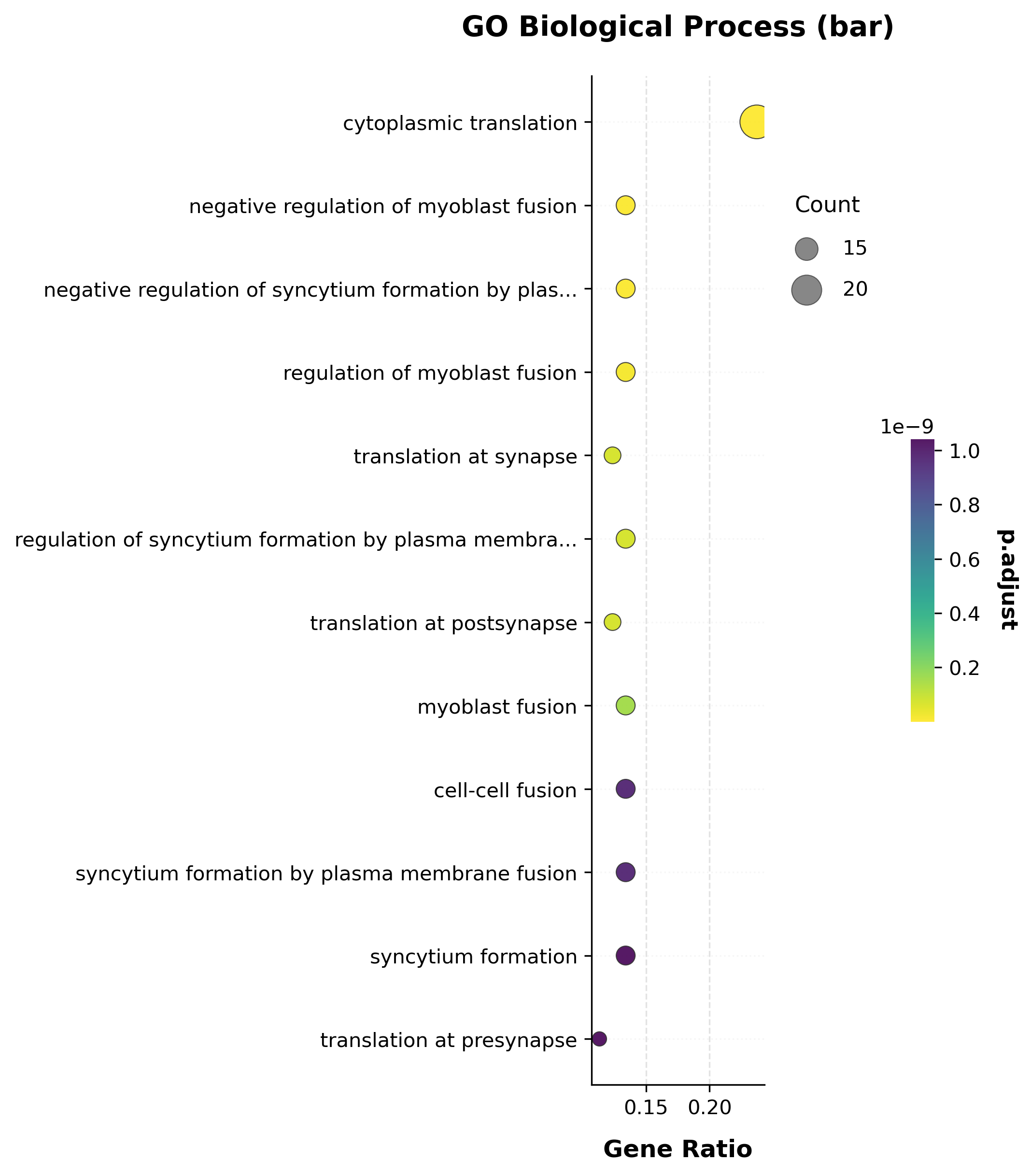
0	cytoplasmic translation (GO:0002181)	23	0.237113	3.700163e-17	2.495390e-13
1	negative regulation of myoblast fusion (GO:190...	13	0.134021	1.380523e-15	4.655122e-12
2	negative regulation of syncytium formation by ...	13	0.134021	2.655028e-15	5.968503e-12
3	regulation of myoblast fusion (GO:1901739)	13	0.134021	1.184686e-14	1.997380e-11
4	translation at synapse (GO:0140241)	12	0.123711	7.259096e-14	7.073882e-11
6	translation at postsynapse (GO:0140242)	12	0.123711	7.259096e-14	7.073882e-11
5	regulation of syncytium formation by plasma me...	13	0.134021	7.342405e-14	7.073882e-11
7	myoblast fusion (GO:0007520)	13	0.134021	1.860772e-13	1.568630e-10
8	cell-cell fusion (GO:0140253)	13	0.134021	1.443489e-12	9.734891e-10
9	syncytium formation by plasma membrane fusion ...	13	0.134021	1.443489e-12	9.734891e-10

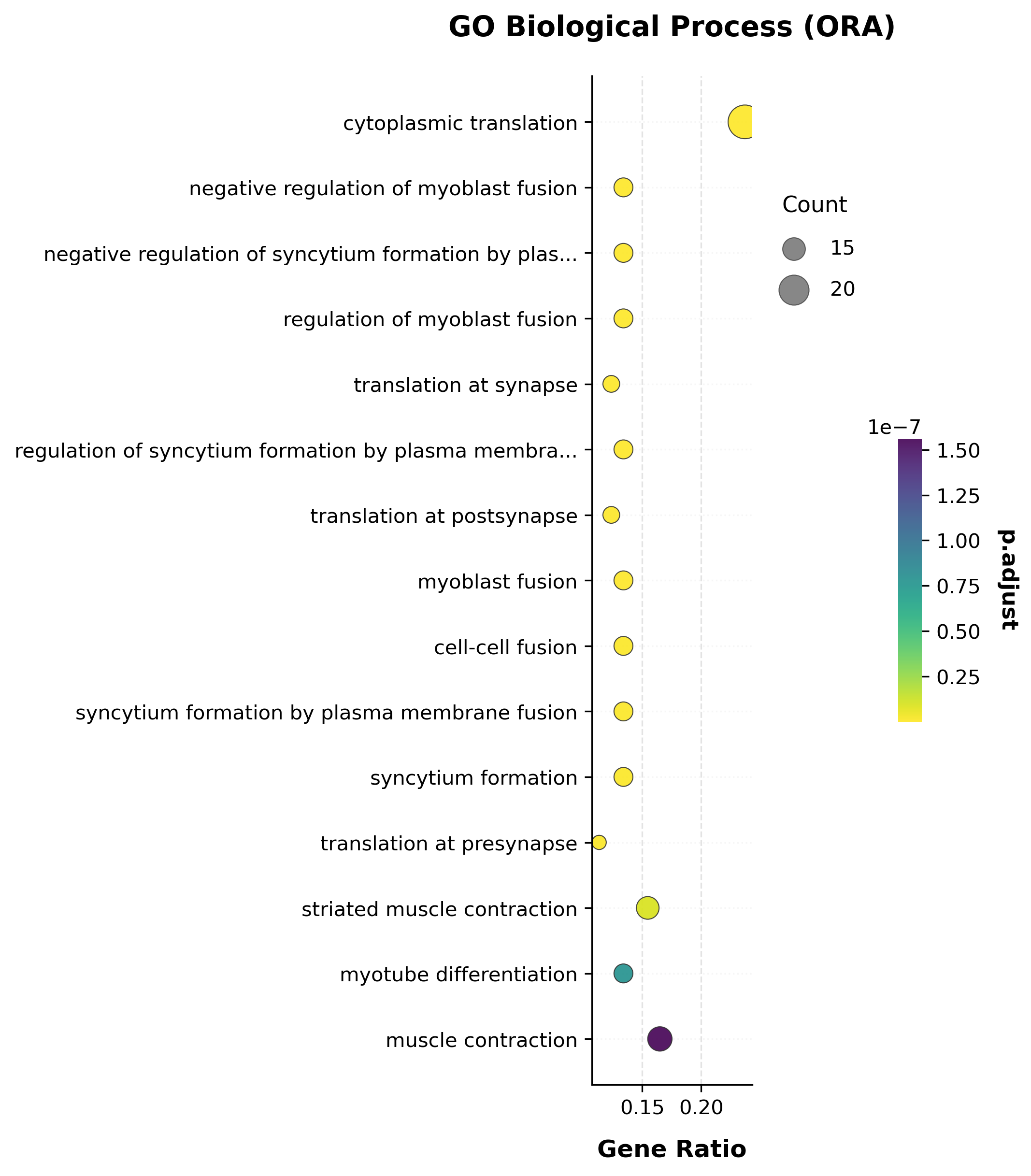
Several ribosomal-protein genes (Rpl37, Rpl35, Rpl37a, Rpl38, Rps19, …) are in the candidate list, so “cytoplasmic translation” comes out as the top term — unlike the per-gene DE p-values, gene-set-level ORA here has genuine, well-powered signal.

KEGG pathways

kegg_res = scat.run_kegg(
    candidate_genes,
    organism="mouse",
    adata=adata_norm,
    return_all=True,
)
kegg_res.sort_values("pvalue").head(10)[["Term", "Count", "pvalue", "p.adjust"]]

	Term	Count	pvalue	p.adjust
0	Ribosome(mmu03010)	21	4.654655e-18	9.402402e-16
2	Parkinson disease(mmu05012)	7	9.762118e-03	6.892085e-01
1	Oxidative phosphorylation(mmu00190)	7	1.023577e-02	6.892085e-01
193	Alzheimer disease(mmu05010)	7	2.363543e-02	1.000000e+00
32	Bile secretion(mmu04976)	3	2.908569e-02	1.000000e+00
201	ABC transporters(mmu02010)	2	5.766020e-02	1.000000e+00
66	Focal adhesion(mmu04510)	6	6.453936e-02	1.000000e+00
38	Cardiac muscle contraction(mmu04260)	3	7.023010e-02	1.000000e+00
72	Glioma(mmu05214)	3	7.808674e-02	1.000000e+00
169	Small cell lung cancer(mmu05222)	3	9.056147e-02	1.000000e+00

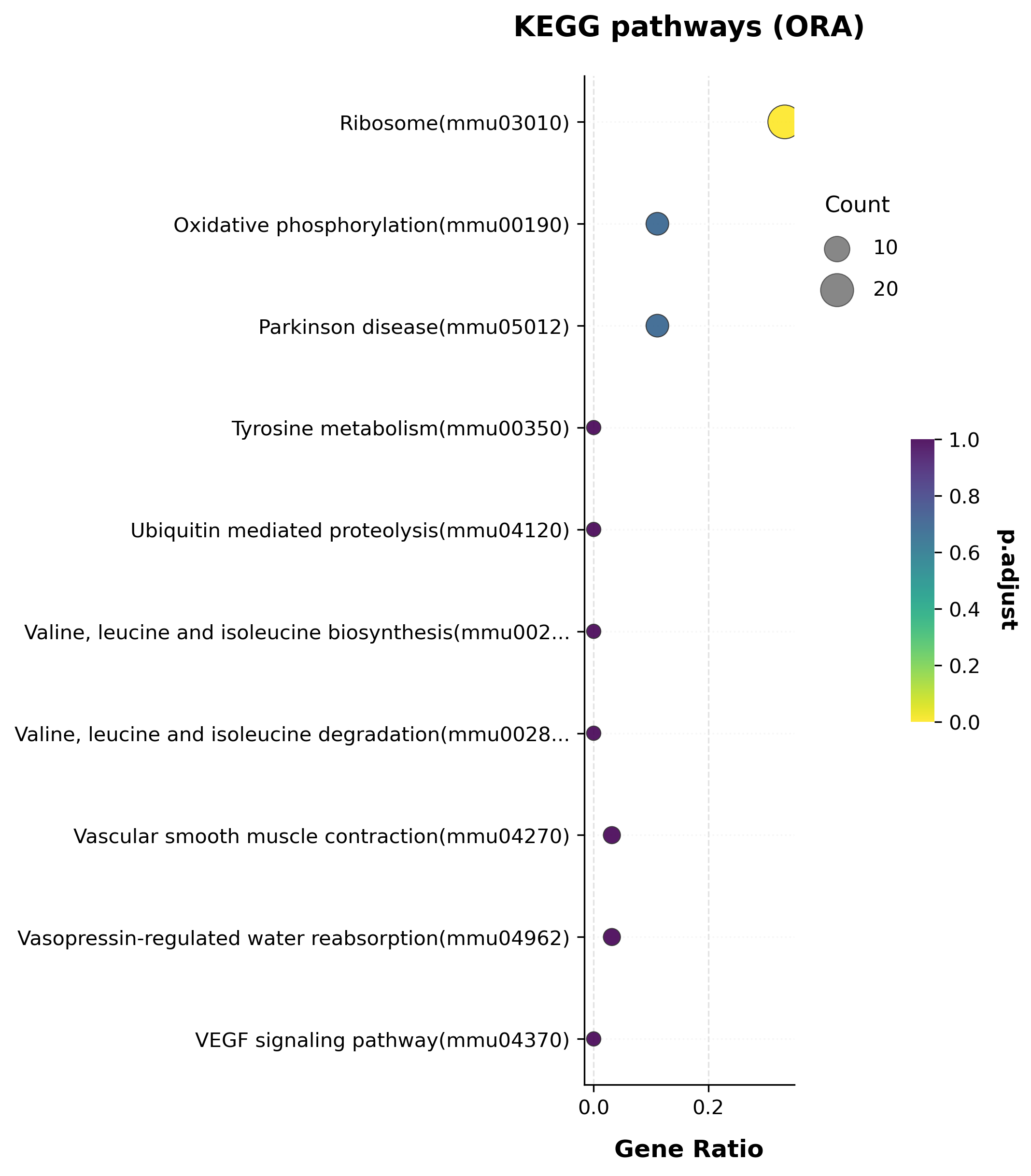
“Ribosome” is overwhelmingly the top KEGG hit here (p.adjust ≈ 1e-15) — consistent with the GO result above.

GO, all three ontologies at once (ontology="ALL")

go_all = scat.run_go(
    candidate_genes,
    ontology="ALL",
    organism="mouse",
    adata=adata_norm,
    return_all=True,
    adjust_across_all=True,  # single BH correction across BP+CC+MF combined
)
print("ontologies covered:", list(go_all.attrs["per_ontology_attrs"].keys()))
go_all.sort_values("pvalue").head(6)[["Term", "Count", "pvalue", "p.adjust"]]

ontologies covered: ['BP', 'CC', 'MF']

	Term	Count	pvalue	p.adjust
0	cytoplasmic translation (GO:0002181)	23	3.700163e-17	2.495390e-13
1	negative regulation of myoblast fusion (GO:190...	13	1.380523e-15	4.655122e-12
2	negative regulation of syncytium formation by ...	13	2.655028e-15	5.968503e-12
3	regulation of myoblast fusion (GO:1901739)	13	1.184686e-14	1.997380e-11
6	translation at postsynapse (GO:0140242)	12	7.259096e-14	7.073882e-11
5	translation at synapse (GO:0140241)	12	7.259096e-14	7.073882e-11

Pre-ranked GSEA

run_gsea takes a full ranked gene list (here, logFC from the Wilcoxon DE result) rather than a fixed candidate cutoff — every gene contributes, weighted by its rank.

Note

nperm controls the permutation-based null distribution; we use a modest nperm=100 here to keep this tutorial cell fast (real run: ~27s). For a manuscript, prefer a larger nperm (≥1000). Roughly 88% of genes in this ranked list share tied logFC values (a side effect of the small-n design above), which run_gsea warns about — tie-breaking within those ranks is arbitrary, so treat exact NES values here as illustrative rather than final.

ranked = de_wilcoxon["logFC"].sort_values(ascending=False)
gsea_res = scat.run_gsea(
    ranked_genes=ranked,
    gene_sets="GO_Biological_Process",
    organism="mouse",
    nperm=100,
    min_size=15,
)
gsea_res.sort_values("p.adjust")[["Term", "NES", "pvalue", "p.adjust", "leading_edge"]].head(10)

2026-07-05 11:40:29,063 [WARNING] Duplicated values found in preranked stats: 87.82% of genes
The order of those genes will be arbitrary, which may produce unexpected results.

	Term	NES	pvalue	p.adjust	leading_edge
0	urogenital system development (GO:0001655)	-2.180388	0.0	0.079007	Igf1;Acd;Osr1;Sulf1;Serpinf1;Acvr1
3	cerebral cortex radially oriented cell migrati...	-2.063498	0.0	0.102709	Bmerb1;Lamb1;Dcx;Fbxo45;Reln;Col3a1
4	regulation of fibroblast growth factor recepto...	-2.013076	0.0	0.116930	Smoc2;Runx2;Sulf1;Wnt4
2	diterpenoid metabolic process (GO:0016101)	-2.074478	0.0	0.121144	Prmt3;Dgat1;Aldh1a1;Rbp4;Dhrs4;Cyp1b1
5	telencephalon glial cell migration (GO:0022030)	-1.977310	0.0	0.137698	Bmerb1;Lamb1;Dcx;Reln;Col3a1
6	cerebral cortex radial glia-guided migration (...	-1.977310	0.0	0.137698	Bmerb1;Lamb1;Dcx;Reln;Col3a1
1	fibroblast growth factor receptor signaling pa...	-2.077310	0.0	0.181716	Sos1;Smoc2;Runx2;Sulf1;Wnt4;Fgfr2;Fgf9;Ccn2;Fg...
9	negative regulation of reproductive process (G...	-1.914572	0.0	0.205418	Igf1;Shb;Sulf1;Ptgds;Serpinf1;Wnt4
8	negative regulation of release of cytochrome c...	-1.915757	0.0	0.228242	Igf1
14	chondrocyte development (GO:0002063)	-1.863570	0.0	0.243341	Runx2;Sulf1

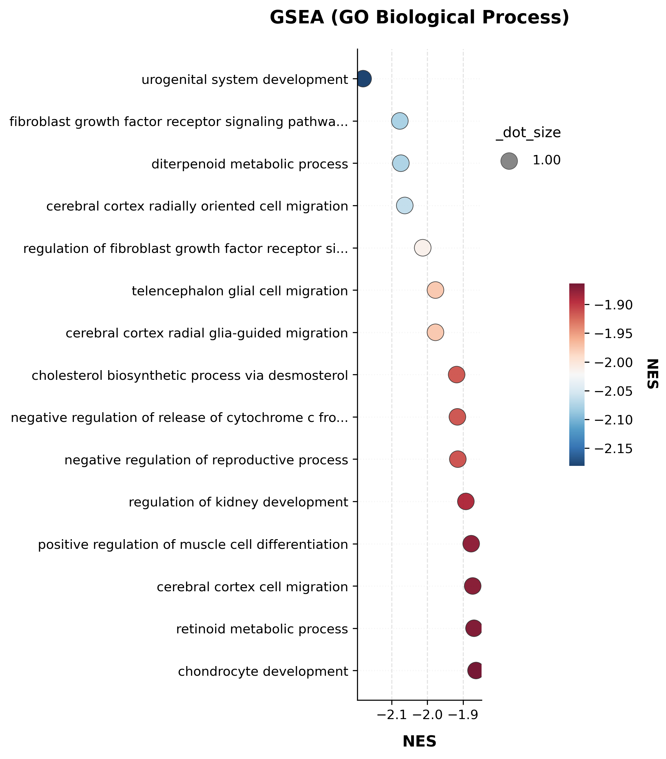
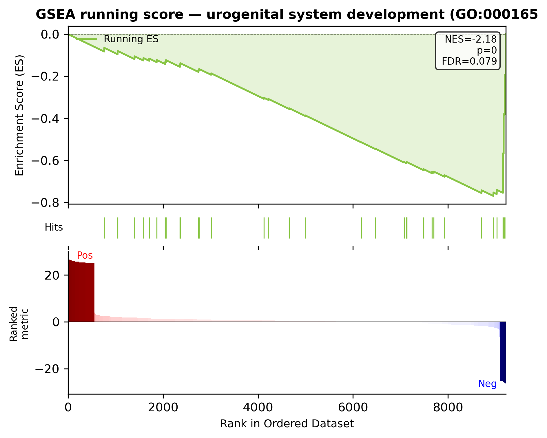
Note

Both scat.pl.gseaplot(...) (the running-sum plot) and scat.pl.enrich_dotplot(gsea_res, x="NES", ...) are shown below. An earlier draft of this tutorial found these calls effectively hung (>1 minute, no error) on a real, thousands-of-terms GSEA result. The root cause turned out to be a real scATrans performance bug, since fixed: run_gsea stored gseapy’s full per-term running-enrichment-score curves in gsea_res.attrs["gsea_details"], and pandas deep-copies .attrs on essentially every DataFrame operation (.head(), .copy(), slicing) via NDFrame.__finalize__ — for a genome-wide ranked list against thousands of gene sets that is tens of millions of floats being deep-copied on every such call. See CHANGELOG.md for the fix (the payload is now wrapped so its __deepcopy__ is an O(1) identity return).

scat.pl.enrich_dotplot(gsea_res, top_n=15, x="NES", color_by="NES", title="GSEA (GO Biological Process)");

top_term = gsea_res.iloc[0]["Term"]
scat.pl.gseaplot(ranked, gsea_res, term=top_term, title=f"GSEA running score — {top_term[:40]}");

simplified_jaccard = scat.simplify_enrichment(
    go_res, method="jaccard", similarity_cutoff=0.5, min_count=3,
)
print(f"jaccard: {len(go_res)} -> {len(simplified_jaccard)} terms")

simplified_denester = scat.simplify_enrichment(
    go_res, method="pathway_denester", min_count=3,
)
print(f"pathway_denester: {len(go_res)} -> {len(simplified_denester)} terms")

jaccard: 6744 -> 162 terms
pathway_denester: 6744 -> 130 terms

Comparing gene sets: compare_enrichment + concat_compare_results

compare_enrichment runs ORA across several named gene lists at once (clusterProfiler’s compareCluster style) and returns a single table with a Cluster column — exactly the shape enrich_upsetplot / enrich_vennplot expect. Here we compare the up- vs. down-regulated candidate genes.

cmp_res = scat.compare_enrichment(
    {"up": candidate_genes, "down": down_genes},
    organism="mouse",
    gene_sets="GO_Biological_Process",
    adata=adata_norm,
)
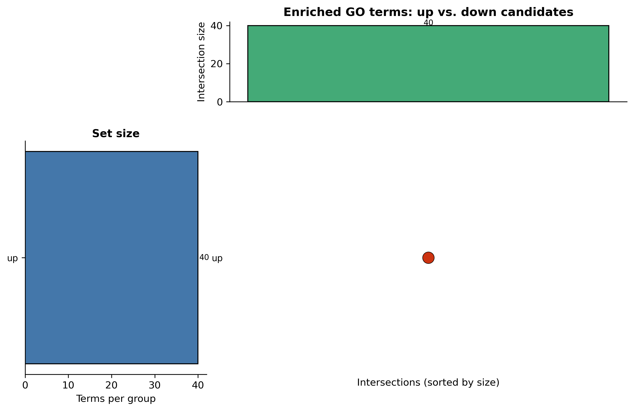
cmp_res["Cluster"].value_counts()

Cluster
up    47
Name: count, dtype: int64

concat_compare_results does the same thing when you already have separate result tables in hand (e.g. combining our GO and KEGG results above into one comparable table):

concat_res = scat.concat_compare_results({"GO": go_res, "KEGG": kegg_res})
concat_res["Cluster"].value_counts()

Cluster
GO      6744
KEGG     202
Name: count, dtype: int64

Exporting results

save_enrichment_report writes CSV/TSV/Excel + a metadata JSON (gene-set provenance, universe info, package version); expand_enrichment_genes pivots to one row per gene for network/follow-up analyses. We write to a scratch temp directory here rather than into the docs tree.

import tempfile, os

tmpdir = tempfile.mkdtemp()
saved_paths = scat.save_enrichment_report(
    kegg_res,
    prefix=os.path.join(tmpdir, "kegg_demo"),
    save_excel=True, save_csv=True, save_tsv=True,
    save_metadata=True, save_term_gene_table=True,
)
saved_paths

{'results_csv': '/tmp/tmplqv4ijao/kegg_demo_results.csv',
 'term_gene_table_csv': '/tmp/tmplqv4ijao/kegg_demo_term_gene_table.csv',
 'results_tsv': '/tmp/tmplqv4ijao/kegg_demo_results.tsv',
 'term_gene_table_tsv': '/tmp/tmplqv4ijao/kegg_demo_term_gene_table.tsv',
 'metadata_json': '/tmp/tmplqv4ijao/kegg_demo_metadata.json',
 'results_xlsx': '/tmp/tmplqv4ijao/kegg_demo_results.xlsx'}

long_table = scat.expand_enrichment_genes(kegg_res)
print(long_table.shape)
long_table.head()

(146, 14)

	Term	Description	Gene	Count	GeneRatio	GeneRatio_str	BgRatio	BgRatio_str	FoldEnrichment	RichFactor	Overlap	pvalue	p.adjust	TermSize
0	Ribosome(mmu03010)		Rpl14	21	0.333333	21/63	0.029197	84/2877	11.416667	0.25	21/84	4.654655e-18	9.402402e-16	84
1	Ribosome(mmu03010)		Rpl18a	21	0.333333	21/63	0.029197	84/2877	11.416667	0.25	21/84	4.654655e-18	9.402402e-16	84
2	Ribosome(mmu03010)		Rpl21	21	0.333333	21/63	0.029197	84/2877	11.416667	0.25	21/84	4.654655e-18	9.402402e-16	84
3	Ribosome(mmu03010)		Rpl23a	21	0.333333	21/63	0.029197	84/2877	11.416667	0.25	21/84	4.654655e-18	9.402402e-16	84
4	Ribosome(mmu03010)		Rpl26	21	0.333333	21/63	0.029197	84/2877	11.416667	0.25	21/84	4.654655e-18	9.402402e-16	84

Plotting gallery

Every scat.pl.* function below accepts ax=, save_path=, show=, figsize=, and use_style= for embedding in multi-panel publication figures (see Visualization).

Volcano plots (3 styles)

scat.pl.volcano_plot(de_wilcoxon, style="auto", top_n=10, title="Volcano — auto (legacy) style");

scat.pl.volcano_plot(
    de_wilcoxon, style="ggvolcano", top_n=10, logfc_cutoff=0.5, pval_cutoff=0.2,
    title="Volcano — ggVolcano style",
);

scat.pl.volcano_plot(de_wilcoxon, style="gradual", top_n=10, title="Volcano — gradual (FDR gradient) style");

Enrichment dot plots and bar plot

scat.pl.enrich_dotplot(go_res, top_n=15, title="GO Biological Process (ORA)");

scat.pl.enrich_dotplot(kegg_res, top_n=10, title="KEGG pathways (ORA)");

scat.pl.enrich_barplot(go_res, top_n=12, title="GO Biological Process (bar)");

UpSet and Venn: comparing up- vs. down-regulated enrichment

Built for compare_enrichment/concat_compare_results output (a Cluster column identifies each group).

scat.pl.enrich_upsetplot(cmp_res, pval_cutoff=0.05, title="Enriched GO terms: up vs. down candidates");

scat.pl.enrich_vennplot(cmp_res, pval_cutoff=0.05, title="Enriched GO terms: up vs. down candidates");

Heatmap of top candidate genes

scat.pl.active_genes_heatmap(adata_norm, candidate_genes[:15], groupby="condition");

Not applicable here

comet_plot, bias_diagnostic_plot, active_score_rankplot, velocity_phase_portraits, and gamma_shrinkage_plot all require active_score/unspliced_excess_*/effective_gamma columns that only exist on the velocity-aware active_score path — see the sibling tutorial Active Transcription Scoring on Real Spinal Cord Injury Data for those.

Recap

Without ever touching a spliced/unspliced layer, this notebook covered:

• Three DE backends (de_method="wilcoxon", use_pseudobulk=True + PyDESeq2, use_memento_de=True) on the same real SCI vs. UN comparison.

• Honest reporting of low per-gene DE power at n=3/group, with an exploratory-ranking workaround.

• The full enrichment toolkit: run_enrichment, run_kegg, run_go(ontology="ALL"), run_gsea, simplify_enrichment (both methods), compare_enrichment / concat_compare_results, and the export helpers.

• The plotting gallery: volcano (3 styles), enrichment dot/bar plots (including the GSEA NES dotplot and running-score plot), UpSet/Venn comparison plots, and a marker-gene heatmap.

See also: Standalone Differential Expression (no velocity data required), Functional Enrichment, Visualization, Statistical Guidance & Reporting Checklist, References & Data Sources, and Active Transcription Scoring on Real Spinal Cord Injury Data if your data does have spliced/unspliced layers.