Active Transcription Scoring on Real Spinal Cord Injury Data

This tutorial runs the full active_score workflow — the velocity-aware path for data with spliced/unspliced (or mature/nascent) layers — on a real dataset: endothelial cells (EC) from adult mouse spinal cord, comparing uninjured controls (UN, 3 replicates) against spinal cord injury (SCI, 3 replicates).

The data are a subset of:

Squair, J.W., Gautier, M., Kathe, C., Anderson, M.A., James, N.D., Hutson, T.H., Hudelle, R., Qaiser, T., Matson, K.J.E., Barraud, Q., Levine, A.J., La Manno, G., Skinnider, M.A., Courtine, G. (2021). Confronting false discoveries in single-cell differential expression. Nature Communications 12, 5692. DOI: 10.1038/s41467-021-25960-2 (GEO GSE165003). See References & Data Sources for the full citation.

Note

This choice of dataset is not an accident. Squair et al. (2021) is about the false-discovery risk of treating single cells as independent replicates in differential expression — exactly the pseudoreplication problem that motivates scATrans’s use_pseudobulk, use_mixed_model, and use_permutation machinery. We will see this play out directly on real data below: a small (3 vs. 3 sample) design has genuinely limited power, and the honest result is that few or no genes clear a strict FDR threshold. We show that outcome as-is rather than manufacturing a cleaner-looking example.

What active_score computes: for each gene, a composite score combining (1) standard differential expression (logFC, adjusted p-value) with (2) a reference-gamma unspliced excess term — how much more unspliced/nascent RNA a gene shows in the target group than expected from a reference-group U/S ratio — after optional bias correction for gene length and intron count. The result is a ranking heuristic, not a p-value; see Statistical Guidance & Reporting Checklist.

%matplotlib inline

import sys
sys.path.insert(0, "../../src")  # use the in-repo scatrans, not any installed copy

import warnings
warnings.filterwarnings("ignore")

import numpy as np
import pandas as pd
import scanpy as sc
import scatrans as scat

print("scatrans", scat.__file__)
sc.settings.verbosity = 1

scatrans /home/lieber/scATrans-main/docs/tutorials/../../src/scatrans/__init__.py

Load the data

EC.h5ad already contains spliced / unspliced layers (plus kb_python’s mature / nascent / ambiguous, which scATrans does not need here since spliced / unspliced are already correctly named).

adata = sc.read_h5ad("../../EC.h5ad")
adata

AnnData object with n_obs × n_vars = 177 × 26451
    obs: 'n_genes_by_counts', 'log1p_n_genes_by_counts', 'total_counts', 'log1p_total_counts', 'pct_counts_in_top_50_genes', 'pct_counts_in_top_100_genes', 'pct_counts_in_top_200_genes', 'pct_counts_in_top_500_genes', 'condition', 'sample', 'GSM_ID', 'total_counts_mt', 'pct_counts_mt', 'n_genes', 'doublet_score', 'predicted_doublet'
    var: 'gene_symbol', 'mt', 'n_cells_by_counts', 'mean_counts', 'pct_dropout_by_counts', 'total_counts', 'n_cells'
    uns: 'sample_colors', 'scrublet'
    layers: 'ambiguous', 'mature', 'nascent', 'spliced', 'unspliced'

adata.obs[["condition", "sample", "GSM_ID"]].value_counts().sort_index()

condition  sample  GSM_ID    
SCI        rep1    GSM5024314    35
           rep2    GSM5024315    23
           rep3    GSM5024316    37
UN         rep1    GSM5024317    27
           rep2    GSM5024318    38
           rep3    GSM5024319    17
Name: count, dtype: int64

Six real biological samples: 3 uninjured (UN) and 3 spinal-cord-injury (SCI) mice, GSM-labeled individually. Note that the sample labels (rep1/rep2/rep3) are reused across conditions but refer to different animals (different GSM_ID) — not a paired/blocked design. This is exactly the case scATrans’s default (non-paired) replicate handling is built for.

print("layers:", list(adata.layers.keys()))
print("X is raw counts:", np.allclose(adata.X.data, np.round(adata.X.data)), "max =", adata.X.max())

layers: ['ambiguous', 'mature', 'nascent', 'spliced', 'unspliced']
X is raw counts: True max = 488.0

Quality control

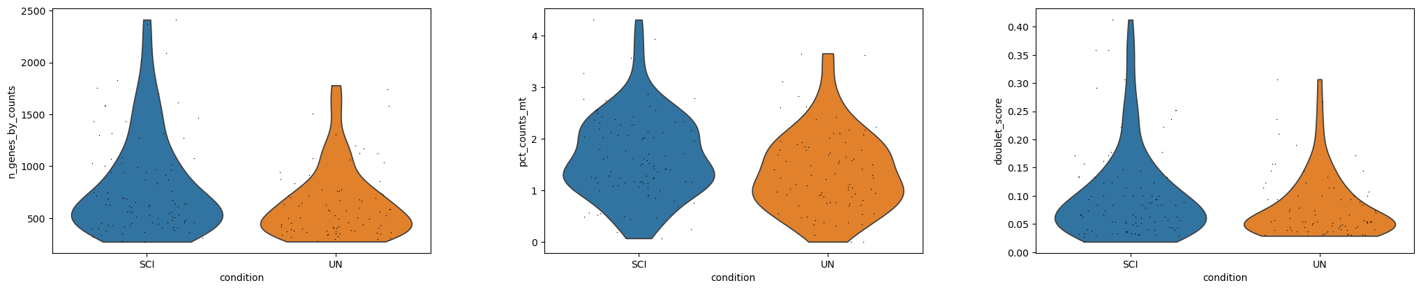
The object already carries QC metrics computed upstream (pct_counts_mt, doublet_score, predicted_doublet, n_genes_by_counts). We inspect them and apply light standard filters.

sc.pl.violin(
    adata,
    ["n_genes_by_counts", "pct_counts_mt", "doublet_score"],
    groupby="condition",
    jitter=0.3,
    multi_panel=True,
)

n_before = adata.n_obs
adata = adata[~adata.obs["predicted_doublet"]].copy()
adata = adata[adata.obs["pct_counts_mt"] < 20].copy()
adata = adata[adata.obs["n_genes_by_counts"] > 200].copy()
sc.pp.filter_genes(adata, min_cells=3)
print(f"cells: {n_before} -> {adata.n_obs}")
print(f"genes retained (>=3 cells): {adata.n_vars}")

cells: 177 -> 177
genes retained (>=3 cells): 9221

This particular dataset was already well curated upstream: none of the 177 cells are dropped by the doublet / mitochondrial / gene-count filters. The gene filter does matter, reducing the universe from 26,451 to the ~9.2k genes detected in at least 3 cells.

ufrac = scat.qc.unspliced_global(adata)
print(f"global unspliced fraction: {ufrac:.1%}")

global unspliced fraction: 30.2%

~30% unspliced is a healthy value (the package warns above ~50%, which often signals a technical issue such as poor nuclear/cytoplasmic capture). active_score re-runs and records this check automatically.

Preserve raw counts, then attach gene features

store_raw_counts snapshots .X and the spliced/unspliced layers before any normalization, so downstream count-based backends (PyDESeq2, Memento) and enrichment background always have access to the full, unmodified gene set. add_gene_features attaches the bundled mouse gene-length / intron-count table used for optional bias correction.

scat.store_raw_counts(adata, layer="counts", save_raw=False)
adata = scat.add_gene_features(adata, organism="mouse")
adata.var[["gene_length", "intron_number"]].describe()

	gene_length	intron_number
count	9221.000000	9221.000000
mean	12915.754148	10.337599
std	15536.314470	9.969041
min	69.000000	0.000000
25%	4750.000000	4.000000
50%	9072.000000	8.000000
75%	16191.000000	14.000000
max	321806.000000	145.000000

A quick look at cell states (optional, descriptive only)

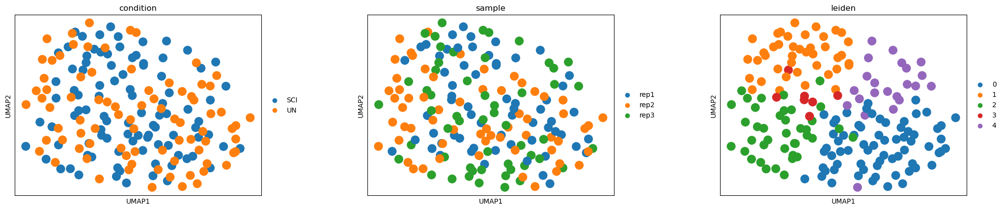
active_score itself works directly on .X plus the spliced/unspliced layers — it does not require a UMAP or clustering. We compute one anyway, purely to visualize how UN and SCI cells separate transcriptionally.

adata_vis = adata.copy()
sc.pp.normalize_total(adata_vis, target_sum=1e4)
sc.pp.log1p(adata_vis)
sc.pp.highly_variable_genes(adata_vis, n_top_genes=2000)
sc.pp.pca(adata_vis, use_highly_variable=True)
sc.pp.neighbors(adata_vis)
sc.tl.umap(adata_vis)
sc.tl.leiden(adata_vis, flavor="igraph", n_iterations=2)
sc.pl.umap(adata_vis, color=["condition", "sample", "leiden"], ncols=3, wspace=0.3)

diagnose_design: let the package tell you what design you have

Before choosing options, run diagnose_design. It inspects cell counts, sample counts, and the global unspliced fraction, and returns concrete warnings and recommendations. It is also called automatically inside active_score whenever sample_col or use_pseudobulk=True is supplied.

diag = scat.diagnose_design(
    adata,
    groupby="condition",
    target_group="SCI",
    reference_group="UN",
    sample_col="sample",
)

print("n_cells (SCI / UN):", diag["n_cells_target"], "/", diag["n_cells_reference"])
print("n_samples (SCI / UN):", diag["n_samples_target"], "/", diag["n_samples_reference"])
print("suggested_preset:", diag["suggested_preset"])
print("workflow_preset:", diag["workflow_preset"])
print("\nwarnings:")
for w in diag["warnings"]:
    print(" -", w)
print("\nrecommendations:")
for r in diag["recommendations"]:
    print(" -", r)

n_cells (SCI / UN): 95 / 82
n_samples (SCI / UN): 3 / 3
suggested_preset: pseudobulk
workflow_preset: pseudobulk_report

warnings:
 - Small number of biological samples per group (target=3, reference=3). Power for detecting differential nascent RNA excess will be limited. Permutation-based FDR is unreliable with so few label shuffles — prefer use_pseudobulk=True without permutation for ranking, then filter_active_genes (preset='pseudobulk') or DE p_adj for significance.

recommendations:
 - With only 3 sample(s) per group, use use_pseudobulk=True (pseudobulk_de_backend='pydeseq2') rather than use_mixed_model=True (requires >=4 samples per group).
 - After running active_score, always inspect adata.uns['scatrans']['diagnostics'] and the distributions in the returned all_results DataFrame before applying cutoffs.

With only 3 biological replicates per group, scATrans itself recommends pseudobulk + PyDESeq2 over a mixed model (which needs ≥4 samples/group) and flags that permutation-based FDR will be unreliable at this sample size. We follow that advice below, and also show what the single-cell heuristic and permutation paths look like for comparison.

Mode A — the one-liner: run_default_pipeline

For a first look, run_default_pipeline scores, filters, and runs GO enrichment in a single call, auto-selecting pseudobulk when enough replicates are present.

result = scat.run_default_pipeline(
    adata,
    groupby="condition",
    target_group="SCI",
    reference_group="UN",
    sample_col="sample",
    organism="mouse",
)
print("auto-selected backend:", result["backend"])
print("filter preset used:", result["filter_preset"])
print("candidates:", len(result["candidates"]))
print("enrichment:", "None (no candidates passed the strict preset)" if result["enrichment"] is None else f"{len(result['enrichment'])} terms")
result["all_results"].sort_values("active_score", ascending=False).head()[["logFC", "p_adj", "active_score"]]

auto-selected backend: {'de_method': 't-test_overestim_var', 'use_pseudobulk': True, 'sample_col': 'sample', 'pseudobulk_de_backend': 'pydeseq2'}
filter preset used: pseudobulk
candidates: 0
enrichment: None (no candidates passed the strict preset)

	logFC	p_adj	active_score
Vcam1	2.211801	0.999513	61.054032
Cobll1	1.093613	0.999513	59.494934
Tmeff2	1.194336	0.999513	58.849826
Pitpnc1	1.018072	0.999513	58.295126
Plcl1	0.962131	0.999513	57.720715

run_default_pipeline auto-selected pseudobulk + PyDESeq2 (because sample_col was supplied with 3 replicates/group) and the matching filter_preset="pseudobulk" — the same honest result as the manual walk-through below: at p_adj < 0.05 on a 3-vs-3 design, zero genes pass, so candidates is empty and enrichment is None (there is nothing to enrich). This is expected, not an error — see Mode C for the exploratory-candidate workaround and a full explanation.

Mode B — manual, single-cell heuristic

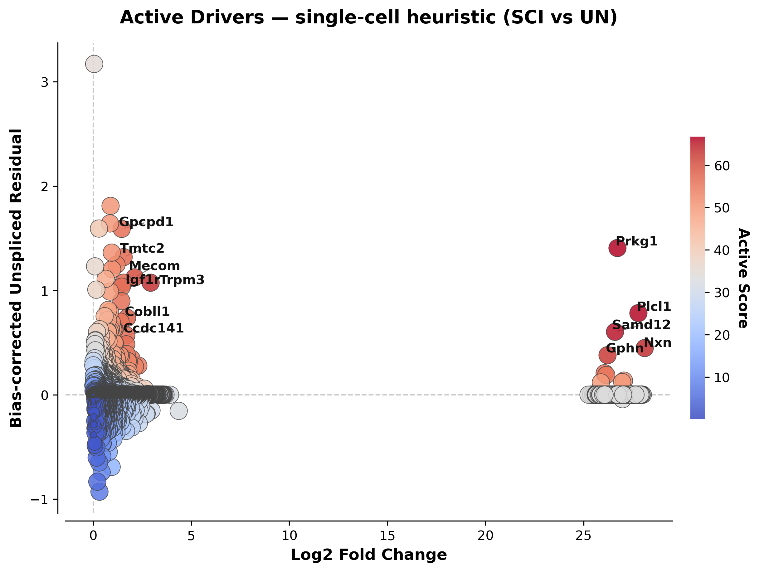
active_score with its defaults runs differential expression per cell (not per pseudobulk sample) and computes the unspliced-excess term directly on single cells.

adata_res, significant, all_results = scat.active_score(
    adata_input=adata,
    groupby="condition",
    target_group="SCI",
    reference_group="UN",
    de_method="wilcoxon",
    show_plot=False,
)
all_results.sort_values("active_score", ascending=False).head(8)[
    ["logFC", "p_adj", "unspliced_excess_residual", "active_score"]
]

	logFC	p_adj	unspliced_excess_residual	active_score
Prkg1	26.726971	0.994983	1.405985	66.727460
Plcl1	27.793922	0.994983	0.782229	66.335979
Samd12	26.600834	0.994983	0.602810	65.628986
Nxn	28.116873	0.994983	0.447306	64.068850
Trpm3	2.930032	0.994983	1.073485	63.555366
Gphn	26.220245	0.994983	0.378836	62.809228
Mecom	2.117509	0.994983	1.124947	60.682844
Cobll1	1.730982	0.994983	0.736788	58.014759

Note

Notice the extreme logFC values (~26-28) on a few genes (e.g. Prkg1, Plcl1, Nxn). This is a well-known artifact of scanpy’s rank_genes_groups log-fold-change estimator when a gene is expressed in very few cells near zero in one group — not evidence of a huge biological effect. active_score’s composite ranking is somewhat robust to this because logFC is only one of three ingredients, but always sanity-check individual genes against raw counts (e.g. with velocity_phase_portraits below) before reporting them. See Statistical Guidance & Reporting Checklist.

print("heuristic-preset candidates:", len(scat.filter_active_genes(all_results, preset="heuristic")))
print("min p_adj across all genes:", all_results["p_adj"].min())

heuristic-preset candidates: 0
min p_adj across all genes: 0.9949828702539322

scat.pl.comet_plot(all_results, top_n=12, title="Active Drivers — single-cell heuristic (SCI vs UN)")

(<Figure size 2400x1800 with 2 Axes>,
 <Axes: title={'center': 'Active Drivers — single-cell heuristic (SCI vs UN)'}, xlabel='Log2 Fold Change', ylabel='Bias-corrected Unspliced Residual'>)

Mode C — pseudobulk + PyDESeq2 (the recommended path here)

This aggregates cells into one pseudobulk profile per (condition, sample) and runs PyDESeq2 — the design diagnose_design recommended above.

adata_res_pb, significant_pb, all_results_pb = scat.active_score(
    adata_input=adata,
    groupby="condition",
    target_group="SCI",
    reference_group="UN",
    use_pseudobulk=True,
    sample_col="sample",
    pseudobulk_de_backend="pydeseq2",
    show_plot=False,
)
all_results_pb.sort_values("active_score", ascending=False).head(10)[
    ["logFC", "p_adj", "unspliced_excess_residual", "active_score"]
]

	logFC	p_adj	unspliced_excess_residual	active_score
Vcam1	2.211801	0.999513	7.739810	61.054032
Cobll1	1.093613	0.999513	23.042433	59.494934
Tmeff2	1.194336	0.999513	11.158579	58.849826
Pitpnc1	1.018072	0.999513	15.865926	58.295126
Plcl1	0.962131	0.999513	16.528507	57.720715
Igf1r	0.899307	0.999513	31.005419	57.308573
Zfp366	1.159273	0.999513	8.128796	56.450931
Mecom	0.866779	0.999513	14.552282	56.212011
Tjp1	0.807648	0.999513	16.418442	55.620784
Rapgef5	0.989955	0.999513	9.047048	55.518645

print("min p_adj (pseudobulk DESeq2):", all_results_pb["p_adj"].min())
print("preset='pseudobulk' candidates:", len(scat.filter_active_genes(all_results_pb, preset="pseudobulk")))
print("built-in `significant` list:", len(significant_pb))

min p_adj (pseudobulk DESeq2): 0.5584481513291821
preset='pseudobulk' candidates: 0
built-in `significant` list: 0

Note

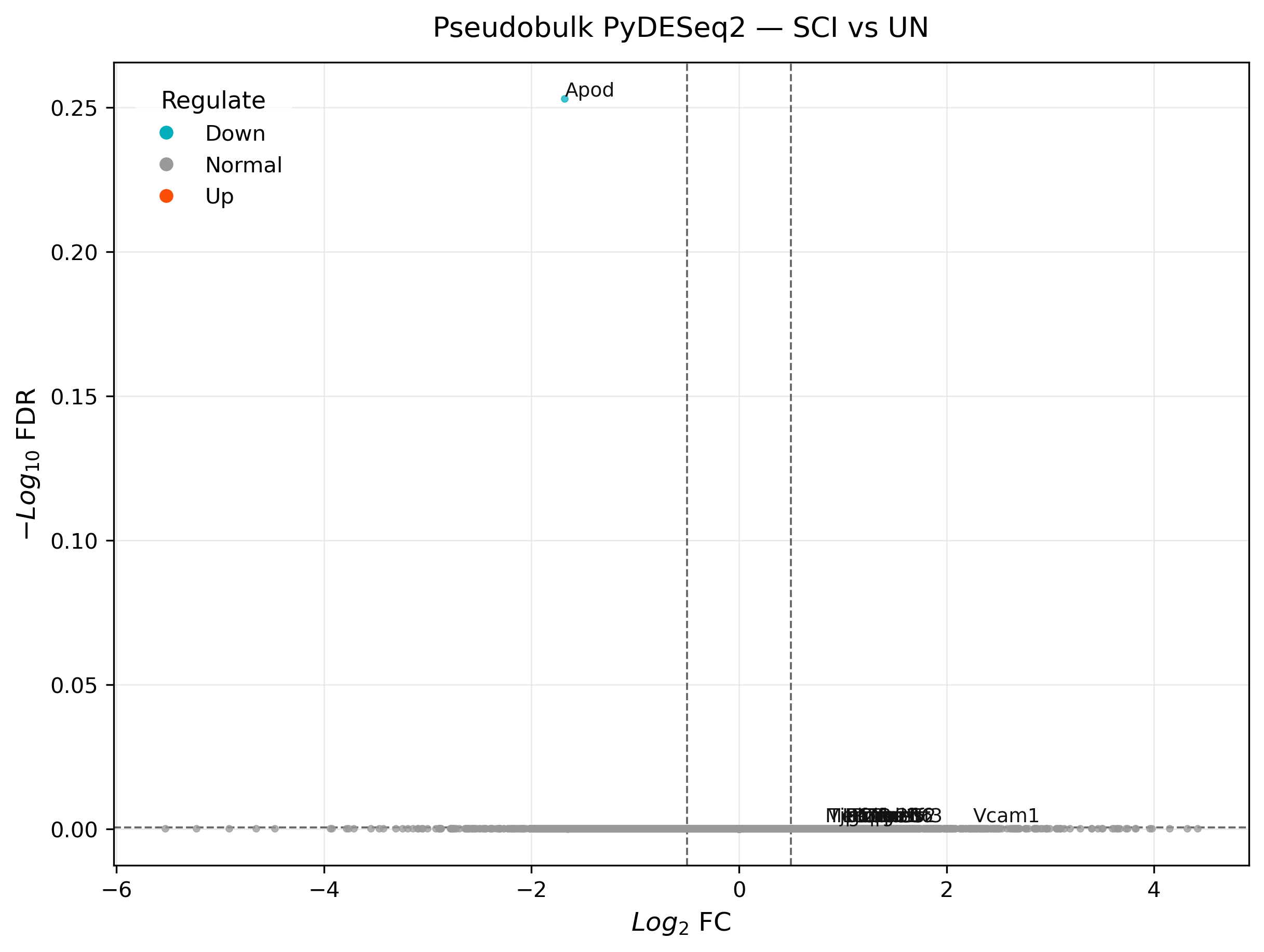
With only 3 vs. 3 pseudobulk samples, no gene clears p_adj < 0.05 here (minimum adjusted p-value ≈ 0.56) — the built-in significant list and the strict preset="pseudobulk" filter are both legitimately empty. This is real, honest low-power biology, not a bug: three replicates per group is thin for genome-wide multiple testing correction. The right move is not to lower the threshold until something turns up, but to treat active_score as a ranking/hypothesis-generating tool and say so plainly in any write-up — see Statistical Guidance & Reporting Checklist.

# Exploratory ranking: effect size + active_score, p-value gate relaxed
# (this is a *ranked candidate list* for hypothesis generation, not a
# p<0.05 confirmatory claim — see the note above).
candidates = scat.filter_active_genes(
    all_results_pb,
    active_score_cutoff=40,
    logfc_cutoff=0.5,
    pval_cutoff=1.0,
)
print("exploratory candidates:", len(candidates))
candidates.sort_values("active_score", ascending=False).head(10)[
    ["logFC", "p_adj", "unspliced_excess_residual", "active_score"]
]

exploratory candidates: 64

	logFC	p_adj	unspliced_excess_residual	active_score
Vcam1	2.211801	0.999513	7.739810	61.054032
Cobll1	1.093613	0.999513	23.042433	59.494934
Tmeff2	1.194336	0.999513	11.158579	58.849826
Pitpnc1	1.018072	0.999513	15.865926	58.295126
Plcl1	0.962131	0.999513	16.528507	57.720715
Igf1r	0.899307	0.999513	31.005419	57.308573
Zfp366	1.159273	0.999513	8.128796	56.450931
Mecom	0.866779	0.999513	14.552282	56.212011
Tjp1	0.807648	0.999513	16.418442	55.620784
Rapgef5	0.989955	0.999513	9.047048	55.518645

scat.pl.volcano_plot(
    all_results_pb,
    style="ggvolcano",
    top_n=12,
    logfc_cutoff=0.5,
    pval_cutoff=0.999,  # relaxed to match the exploratory cutoff above (p_adj min here is ~0.56)
    title="Pseudobulk PyDESeq2 — SCI vs UN",
)

(<Figure size 2400x1800 with 1 Axes>,
 <Axes: title={'center': 'Pseudobulk PyDESeq2 — SCI vs UN'}, xlabel='$Log_2$ FC', ylabel='$-Log_{10}$ FDR'>)

Mode D — permutation-based FDR (single-cell path)

diagnose_design already warned that permutation is unreliable with only 3 samples/group in pseudobulk mode. We instead demonstrate the mechanism on the single-cell heuristic path with a modest n_perm and the fast backend, purely to show how it works — the conclusion is consistent with everything above: still no significant genes at this sample size.

adata_res_perm, significant_perm, all_results_perm = scat.active_score(
    adata_input=adata,
    groupby="condition",
    target_group="SCI",
    reference_group="UN",
    use_permutation=True,
    n_perm=100,
    perm_de_backend="fast",  # exploratory speed; use "same" for manuscript-quality FDR
    show_plot=False,
)
print("significant (permutation FDR):", len(significant_perm))
print(adata_res_perm.uns["scatrans"].get("permutation_approximation_note"))
all_results_perm.sort_values("active_score", ascending=False).head(5)[
    ["logFC", "p_adj", "unspliced_excess_fdr", "active_score"]
]

significant (permutation FDR): 0
For efficiency, unspliced/spliced layers and reference gamma are fixed from the original data. Group labels are shuffled to recompute DE, unspliced excess residual, composite active_score, and unspliced_excess permutation p-values.

	logFC	p_adj	unspliced_excess_fdr	active_score
Plcl1	27.793922	0.498326	0.999048	74.963961
Nxn	28.116873	0.456581	1.000000	73.615214
Prkg1	26.726971	0.587123	0.706809	73.537238
Igf1r	1.549713	0.212572	0.501937	73.407025
Mecom	2.117509	0.347586	0.632578	72.878279

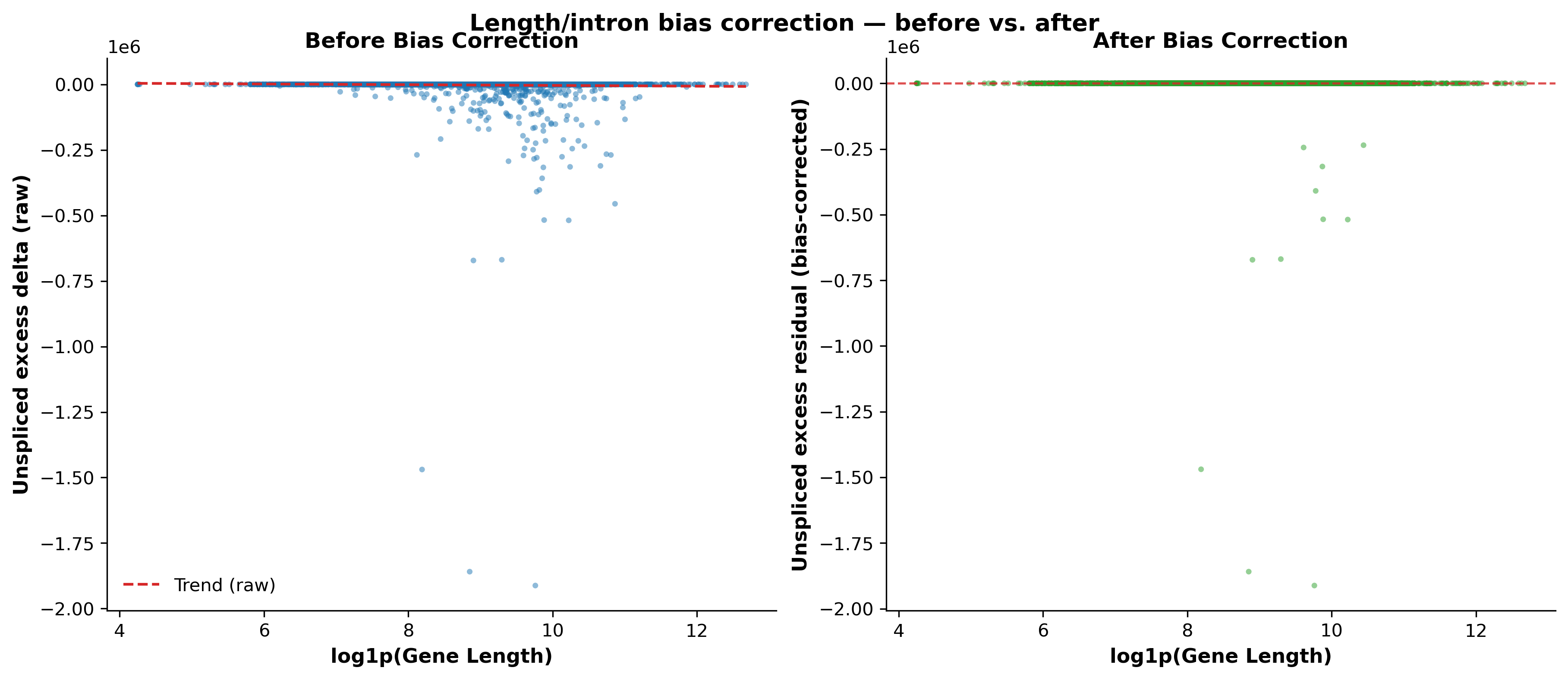
Mode E — reference-gamma robustness and bias-correction diagnostics

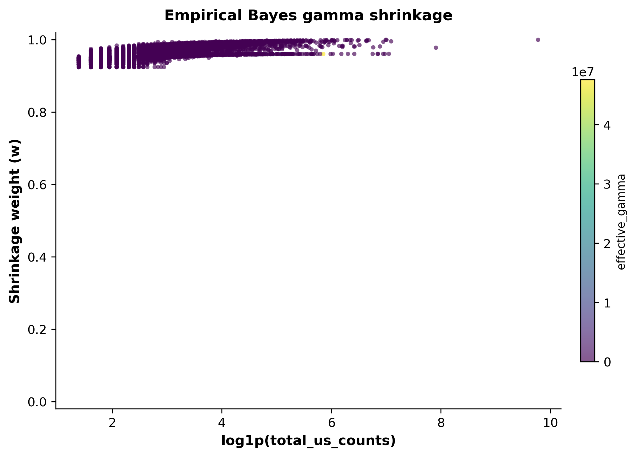
gamma_method="empirical_bayes" shrinks each gene’s reference U/S ratio toward a shared, hierarchically-estimated prior — a more robust option when the reference group is small. show_effective_gamma=True exposes the per-gene shrunk gamma so its behavior can be inspected directly.

adata_res_gb, _, all_results_gb = scat.active_score(
    adata_input=adata,
    groupby="condition",
    target_group="SCI",
    reference_group="UN",
    gamma_method="empirical_bayes",
    show_effective_gamma=True,
    show_plot=False,
)
v = adata_res_gb.uns["scatrans"]["diagnostics"]["velocity"]
print("gamma_prior_mean:", v.get("gamma_prior_mean"))
print("shrinkage_summary:", v.get("shrinkage_summary"))

gamma_prior_mean: -2.1783053057222053
shrinkage_summary: {'mean': 0.9630662745530777, 'q10': 0.94207253767107, 'q25': 0.9508108342897064, 'q50': 0.9590140129606987, 'q75': 0.9786133392259676, 'q90': 0.9873976599591713}

scat.pl.gamma_shrinkage_plot(all_results_gb)

(<Figure size 2100x1500 with 2 Axes>,
 <Axes: title={'center': 'Empirical Bayes gamma shrinkage'}, xlabel='log1p(total_us_counts)', ylabel='Shrinkage weight (w)'>)

scat.pl.bias_diagnostic_plot(all_results_gb, title="Length/intron bias correction — before vs. after")

(<Figure size 3600x1500 with 2 Axes>,
 array([<Axes: title={'center': 'Before Bias Correction'}, xlabel='log1p(Gene Length)', ylabel='Unspliced excess delta (raw)'>,
        <Axes: title={'center': 'After Bias Correction'}, xlabel='log1p(Gene Length)', ylabel='Unspliced excess residual (bias-corrected)'>],
       dtype=object))

Mode F — advanced mode (scVelo moments smoothing)

mode="advanced" uses scVelo’s moments (kNN-smoothed spliced/unspliced means) before computing the group-wise gamma delta, instead of the raw per-cell counts. It is still a reference-gamma excess calculation, not a full dynamical velocity model — just computed on smoothed rather than raw values. Requires pip install "scatrans[advanced]".

adata_res_adv, _, all_results_adv = scat.active_score(
    adata_input=adata,
    groupby="condition",
    target_group="SCI",
    reference_group="UN",
    mode="advanced",
    show_plot=False,
)
all_results_adv.sort_values("active_score", ascending=False).head(5)[
    ["logFC", "p_adj", "active_score"]
]

computing moments based on connectivities
    finished (0:00:00) --> added 
    'Ms' and 'Mu', moments of un/spliced abundances (adata.layers)

	logFC	p_adj	active_score
Plcl1	27.793922	0.498326	74.586539
Prkg1	26.726971	0.587123	73.507546
Nxn	28.116873	0.456581	73.222538
Mecom	2.117509	0.347586	72.813430
Igf1r	1.549713	0.212572	72.749187

Closing the loop: one enrichment pass

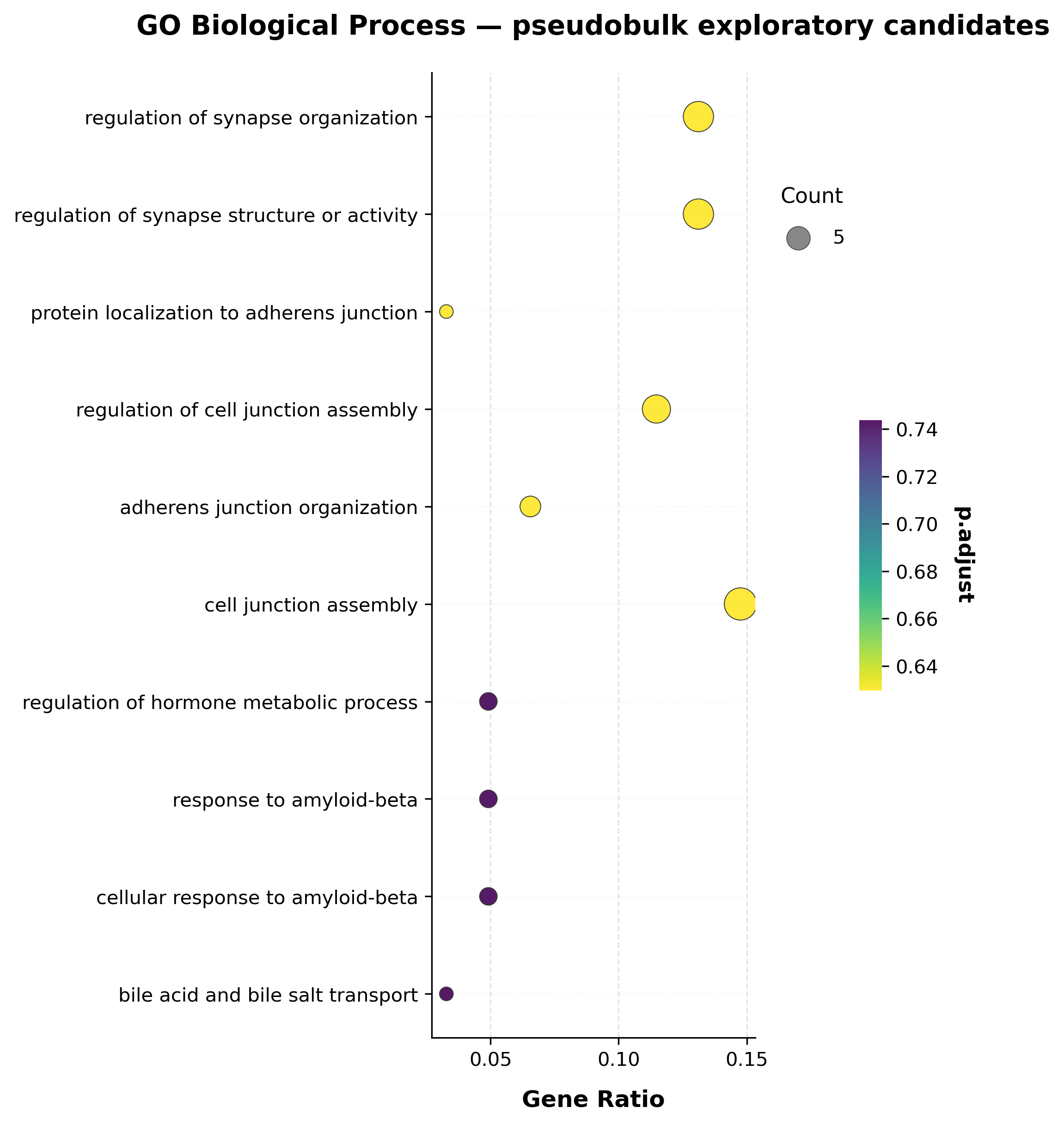
Functional enrichment is covered in full in the companion tutorial, scATrans without spliced/unspliced layers: differential expression + enrichment + plotting (ORA, KEGG, GO all-ontology, GSEA, redundancy reduction, and the full plotting gallery). Here we just run one GO Biological Process over-representation test on the pseudobulk exploratory candidates from Mode C, to close the workflow end to end.

enrich_res = scat.run_enrichment(
    gene_list=candidates.index.tolist(),
    gene_sets="GO_Biological_Process",
    organism="mouse",
    adata=adata,          # uses the full stored gene set (from store_raw_counts) as background
    pval_cutoff=1.0,       # relaxed, consistent with the exploratory candidate list above
)
print(enrich_res.shape)
enrich_res.sort_values("pvalue").head(10)[["Term", "Overlap", "pvalue", "p.adjust"]]

(13, 15)

	Term	Overlap	pvalue	p.adjust
4	adherens junction organization (GO:0034332)	4/33	0.000094	0.629774
0	regulation of synapse organization (GO:0050807)	8/253	0.000505	0.629774
2	protein localization to adherens junction (GO:...	2/5	0.000530	0.629774
5	cell junction assembly (GO:0034329)	9/321	0.000531	0.629774
3	regulation of cell junction assembly (GO:1901888)	7/195	0.000548	0.629774
1	regulation of synapse structure or activity (G...	8/257	0.000560	0.629774
6	regulation of hormone metabolic process (GO:00...	3/25	0.000788	0.742972
8	cellular response to amyloid-beta (GO:1904646)	3/26	0.000886	0.742972
7	response to amyloid-beta (GO:1904645)	3/27	0.000992	0.742972
9	bile acid and bile salt transport (GO:0015721)	2/7	0.001103	0.743692

if len(enrich_res):
    scat.pl.enrich_dotplot(enrich_res, top_n=10, title="GO Biological Process — pseudobulk exploratory candidates")
else:
    print("No enrichment terms to plot.")

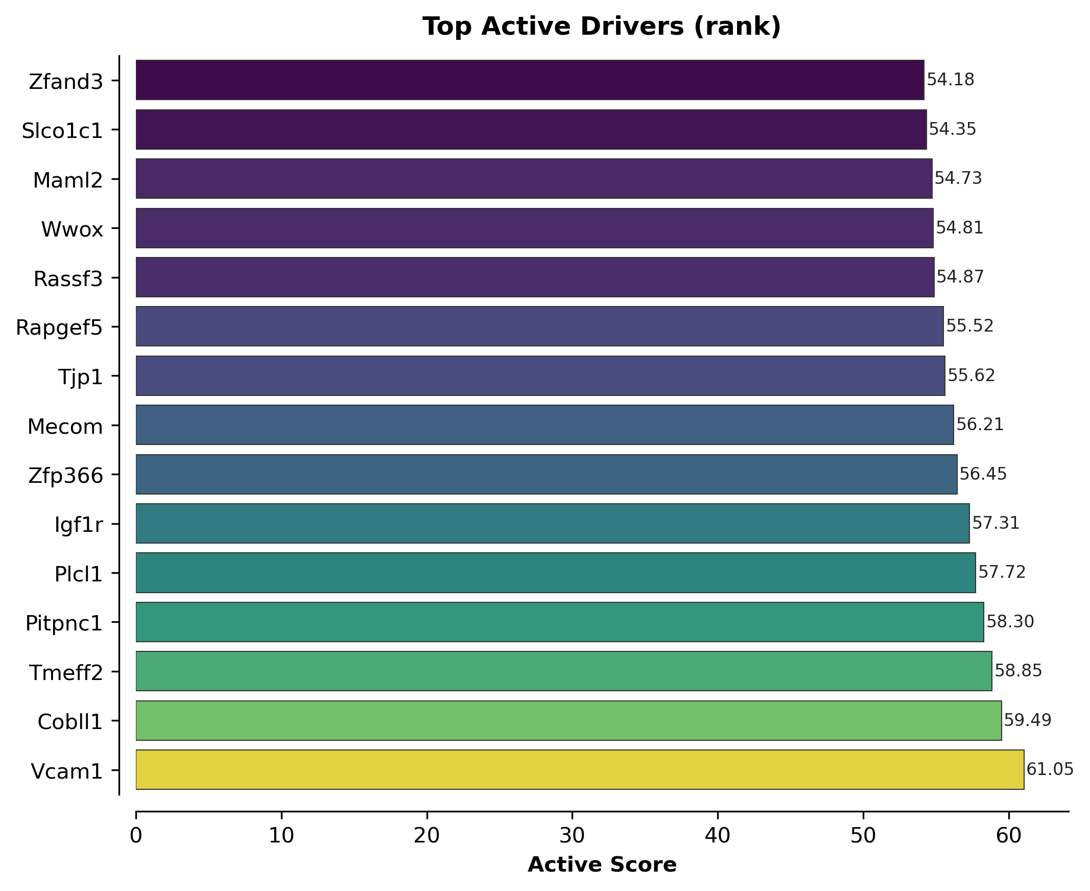
Rank plot and expression heatmap for the top candidates

scat.pl.active_score_rankplot(all_results_pb.sort_values("active_score", ascending=False), top_n=15)

(<Figure size 2100x1710 with 1 Axes>,
 <Axes: title={'center': 'Top Active Drivers (rank)'}, xlabel='Active Score'>)

top_genes = all_results_pb.sort_values("active_score", ascending=False).head(10).index.tolist()
scat.pl.active_genes_heatmap(adata_res_pb, genes=top_genes, groupby="condition")

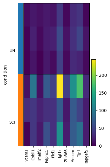
({'heatmap_ax': <Axes: >, 'groupby_ax': <Axes: ylabel='condition'>}, None)

scat.pl.velocity_phase_portraits(adata, genes=top_genes[:4], groupby="condition")

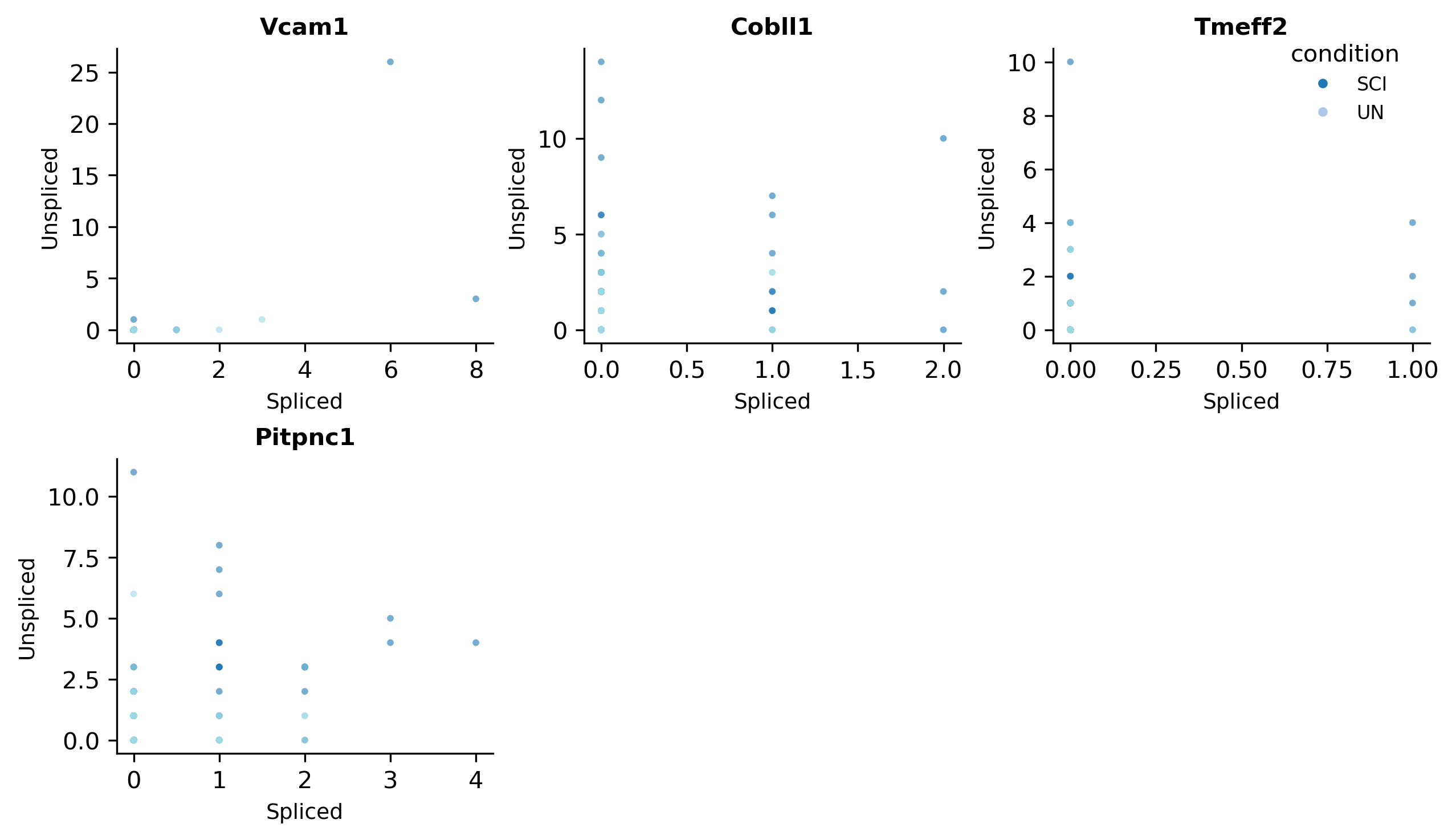
(<Figure size 2520x1440 with 6 Axes>,
 array([<Axes: title={'center': 'Vcam1'}, xlabel='Spliced', ylabel='Unspliced'>,
        <Axes: title={'center': 'Cobll1'}, xlabel='Spliced', ylabel='Unspliced'>,
        <Axes: title={'center': 'Tmeff2'}, xlabel='Spliced', ylabel='Unspliced'>,
        <Axes: title={'center': 'Pitpnc1'}, xlabel='Spliced', ylabel='Unspliced'>,
        <Axes: >, <Axes: >], dtype=object))

Recap

• diagnose_design / recommend_workflow read the experimental design (here: 3 vs. 3 samples, ~30% unspliced) and steer you toward pseudobulk + PyDESeq2 rather than a mixed model or permutation FDR.

• On this real, modestly-powered dataset, strict significance filters (preset="pseudobulk", preset="significant", permutation FDR) all legitimately return no genes — that is the honest answer for a 3 vs. 3 design, not a failure of the tool.

• active_score and filter_active_genes with relaxed, explicit cutoffs still produce a usable ranked candidate list for downstream enrichment and hypothesis generation.

• Always report active_score as a composite heuristic rank, not a p-value — see Statistical Guidance & Reporting Checklist for the full reporting checklist, Optional Advanced Features for every option shown above, and References & Data Sources for the data and method citations.